The useful result was a boundary, not a victory lap.
Early in the draft, the counting estimator was better on the comparison I had built. Later, a jointly fitted model was better. That suggested using both, rather than asking one of them to win everywhere.
There is a change of protagonist to explain first. The model in this race is not the Transformer from the opening installments.
Three Ways to Score a Draft
The Transformer learns hero representations and attention over the supplied lineup. It is flexible, but that flexibility hadn't earned a reliable advantage over counting on the early-pick tests.
The counting estimator starts with observed hero and pair outcomes. It combines individual strength, within-team synergy, and cross-team matchup terms. The stronger version reads bracket-conditioned tables and shrinks noisy estimates toward pooled values. It does not look up an exact ten-hero lineup.
The new structured pairwise model has a similar decomposition, but its roughly 50,000 parameters are fitted jointly by gradient descent. Individual hero effects, teammate-pair effects, opponent-pair effects, and count-dependent weights contribute to one score. The structure is hand-designed; the values are learned. It is not a hand-written hero tier list.
Both pairwise approaches can score combinations they have never seen by composing their parts. The experiment asks which fitting method does that more usefully, not whether counting understands nothing and a network understands everything.
A Measurement That Reaches Further Into the Draft
At depth, exact historical matches for a candidate and its entire context become scarce. I couldn't keep using a direct per-candidate win-rate table and simply turn the "heroes known" knob upward.
Instead, I grouped similar contexts. Heroes were clustered into eight groups using their counter profiles. A context key recorded the groups represented on each team, rather than demanding identical hero IDs.
This is coarsening, not a claim that the grouped heroes are strategically interchangeable. It buys enough observations to compare, at the cost of leaving important differences inside each group.
For each completed match, the evaluator sampled a partial context and revealed one of our remaining heroes as the candidate. This is a synthetic masking experiment, not a reconstruction of which hero that player actually picked next.
The score was within-context concordance: among winning and losing rows in the same group, how often did the estimator rank the winning row higher? Ties count half. Before that comparison, scores were adjusted within groups for a solo-strength baseline. A value of 0.5 is chance; the reported margin is the difference from the bracket-aware counting estimator.
That is a discrimination statistic, not additional games won by following the recommendations.
The experiment used 600,000 sampled matches from the later test partition of the 27.7-million-match snapshot. They were held out from model fitting, but the partition had already informed earlier research. I also revised the acceptance criteria after the original test failed. This is exploratory held-out evidence, not a fresh confirmatory test.
Where the Sign Changes
The chart uses the corrected context key discussed in Part 10. Counts on its horizontal axis describe the request before a candidate is inserted.
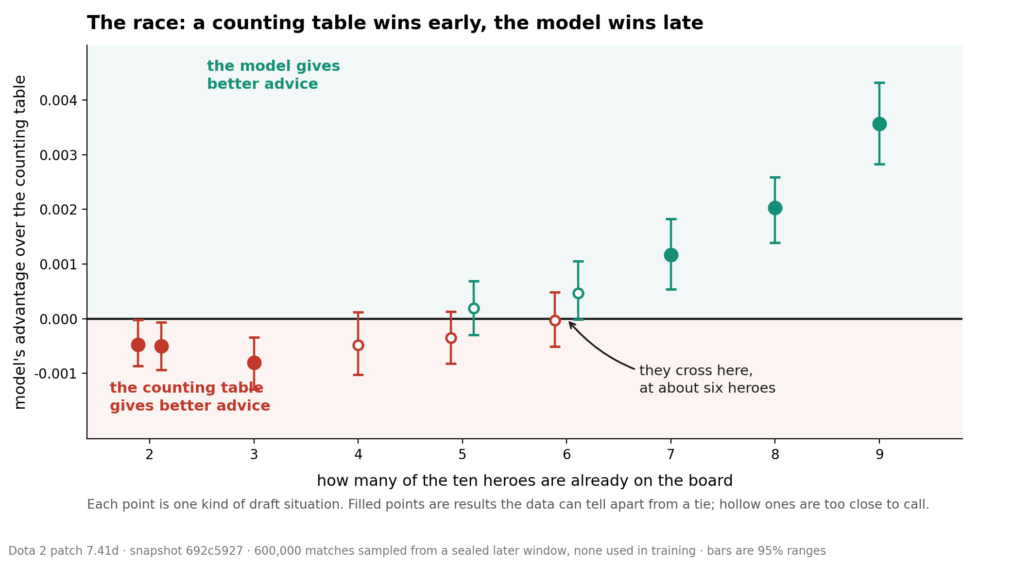
At 1/2 - one of ours and two of theirs already selected - the structured model's concordance margin was about -0.00080. At 4/5, the final pick, it was about +0.00356. The transition was around five or six known heroes, with mixed signs in that region, not a magical universal cutoff.
The measured states represented 80% of the trace-derived request mass. The omitted 20% was 0/0, 0/1, and 1/0: too few usable context groups for this particular interval calculation. The opening requests weren't unimportant or solved perfectly by a table. This instrument simply did not cover them.
The full acceptance test did not pass. Both weighted primary criteria passed, but the no-worse-state guard failed at 0/2, 1/1, and 1/2. Repairing the context key improved one primary verdict; it did not turn the overall failure into a pass.
That failure was compatible with the useful observation: the model should not replace the table everywhere. A switch might preserve the table's early results and use the fitted model later. It still needed to be selected and evaluated as a combined estimator.
What Scaling Didn't Settle
I also compared Transformers of about 1.1, 2.6, and 4.8 million parameters. The recorded counter-ranking diagnostic declined across those three runs, from about 0.689 to 0.604.
I initially described that as "bigger is worse." Subsequent seed checks made that interpretation indefensible as a general result. Three repetitions of one configuration spanned about 0.076 on the diagnostic. The endpoint gap in the size comparison was about 0.085 - larger, not smaller, but of a similar order.
A range across three seeds is not an error bar for every model size, and the comparison did not independently tune each size's training recipe. It supports saying that these larger runs did not show a benefit. It does not establish a monotonic law about capacity, or that the model had exhausted what it could learn.
I've removed the scale chart whose borrowed error bars suggested more certainty than that design supplied. The fitted pairwise model was the more useful line to pursue here, without needing a story about attention always doing the easy job first.
The next step was concrete: select a switching threshold on validation, then measure the combined estimator. Before presenting that result, Part 10 records the measurement failures that changed what I was willing to claim from it.