Best epoch: 8, of 8.
Both of my first Transformer runs on the new dataset ended there. Their best checkpoint was the last one I'd allowed them to produce. That was worth investigating, but it didn't say how much improvement another hour would buy.
The manual sweeps in Part 4 had produced workable settings. Now I had a much larger dataset and a different training setup. I wanted room to compare alternatives without treating each GPU run as a special occasion.
Keep the Ranks, Add the Context
First, the question left by Part 5: should the model know which rank bracket a match belongs to?
I started cheaply, with logistic regression on signed hero indicators: one weight per hero, added for Radiant and subtracted for Dire, plus a side bias. I fitted it both across the training population and separately within each bracket.
On the same Divine test matches, the pooled fit scored 54.99% accuracy and the Divine-only fit scored 55.99%. This was evidence that pooled hero valuations could miss bracket-specific patterns. It wasn't a controlled study of intrinsic predictability across ranks: the bracket datasets differed in size, and these linear models weren't the Transformers from Part 2.
I then trained a Transformer with the bracket as an additional input, rather than discarding higher-ranked games. Both Transformer runs used 21.4 million training matches, the same eight-epoch recipe, and the same validation split. The comparison on 2,671,633 validation matches was:
| Model | Accuracy | Log loss |
|---|---|---|
| Signed hero-indicator logistic regression | 56.24% | 0.68108 |
| Transformer without rank input | 58.90% | 0.66831 |
| Transformer with rank input | 59.14% | 0.66703 |
Log loss scores the predicted probabilities, not just the chosen winner; lower is better. The rank-conditioned run was ahead at each of the eight epochs and finished about a quarter of a percentage point ahead in accuracy. Keeping rank as information was more promising than treating it only as a filter.
These are complete-draft prediction results. They don't yet measure whether the model recommends good picks in an unfinished draft.
Price the Experiment Before Ordering Thirty
The final-epoch result made a longer schedule worth trying, not automatically worth tripling. A subsequent 24-epoch run reached 59.19%, only about 0.05 percentage points above the eight-epoch result.
That run also used mixed precision. And stretching a cosine schedule changes the learning rate throughout training: it isn't the original eight epochs with sixteen more attached. The comparison did not isolate the benefit of extra epochs, much less establish that schedule length was the main bottleneck.
Still, longer runs had to fit inside the search budget. I used 24 epochs per trial and thirty trials as a planning case. At the full-precision epoch times I measured, that meant roughly 59 GPU-hours, before the work outside the epoch loop. Quite a commitment for a list of configurations I expected many of to disappoint me.
Use Less Precision Where It Helps
PyTorch's automatic mixed precision, or AMP, lets suitable operations use a faster 16-bit path while keeping others in full precision. In this setup the stored model parameters remain 32-bit. It isn't a blanket conversion of every number in the program.
The complication is range. Small gradients can underflow in lower precision.
GradScaler multiplies the loss before backpropagation, scaling up the
gradients with it, then removes that scale before the optimizer update. It
adjusts the scale during training and skips updates when it detects overflow.
I already clipped gradients by norm, so the order matters. Clipping a gradient that has been multiplied by 65,536 against its ordinary threshold is not the operation I intended. Unscale first:
scaler.scale(loss).backward()
scaler.unscale_(optimizer)  # Restore the scale that max_norm refers to.
torch.nn.utils.clip_grad_norm_(model.parameters(), max_norm)
scaler.step(optimizer)
scaler.update()
A later matched timing comparison used the refreshed snapshot with 22.2 million training matches. Jobs 178 and 179 ran on the same GPU, with identical settings apart from AMP, for four epochs each. Their mean recorded epoch times were 293.1 seconds in full precision and 138.6 with AMP: roughly 2.1× faster.
Both finished at about 59.00% validation accuracy, with log losses of 0.66766 and 0.66772 respectively. That was a useful sanity check for this configuration, not a guarantee that reduced precision would be harmless in every experiment.
The speedup is for the epoch loop, including its validation work. Loading data, saving artifacts, and the final evaluation suite still cost time outside it.
Use the Queue I Already Built
The scheduler hadn't been idle since Part 3; it had run the Part 4 sweep. What I needed now was to connect the rewritten, snapshot-based training script and expose its new options.
That produced one particularly avoidable delay. I added the AMP option, updated the code on the worker, and kept seeing the old parameter list on the dashboard. The worker was polling successfully. The files were current. I checked the commit again, as though Git might have changed its mind.
The worker discovers the schema once, at startup. Its successful polls were sending the cached list. Restarting it advertised the new option. The contract I'd designed was doing exactly what it said; I'd forgotten which part of it was allowed to remember things.
With that sorted, I could submit a batch and let the worker process it sequentially. No new distributed system was required.
For choosing the configurations, the plan was to use Optuna's Tree-structured Parzen Estimator, or TPE. A grid with ten settings and three values per setting has 59,049 combinations. I did not have that kind of relationship with my GPU.
TPE uses previous trials to fit distributions of configurations associated with better and worse results, then favours candidates with a high ratio of the former density to the latter. It handles the mix of numerical settings and discrete choices I had. That made it a reasonable search strategy, not a measured guarantee that I'd need fewer trials than random search.
What the Budget Buys
The figure below is a planning projection, not a timed thirty-trial search. It assumes 24 epochs at the measured mean rates, uninterrupted GPU availability, and no overhead outside the epoch loop.
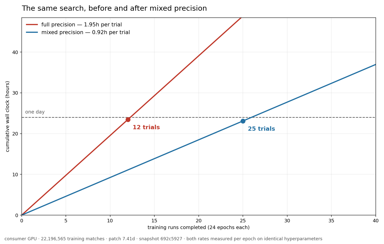
Under those assumptions, thirty trials fall from about 59 hours to 28. Not overnight, and not a promise for every model size. But enough of a change to make controls and repeat runs less tempting to omit from the plan.
The next comparison was about what the model was learning, rather than how fast I could train it. The current baseline used complete drafts. February's early masked-view experiment hadn't validated partial-draft advice either. I could now afford to test that gap instead of assuming an input mask had closed it.