When we left off, I had finished building a small distributed scheduler so I could queue up training jobs without babysitting them. The model was sitting at 56.27% test accuracy on Herald-through-Archon games -- a clean signal, but a weak one. The machinery for pushing it further was finally in place.
I will spare you the agony of describing eighty experiments individually. Here is the dashboard view of how this period actually looked: a column of 25-minute jobs piling up overnight, each spitting out a test accuracy at the bottom, while I slept and ate and did chores and occasionally peeked at my phone. It was the most boring kind of progress, which is the best kind.
But the story of those eighty jobs has a shape, and the shape ends somewhere I genuinely didn't see coming.
Part 1: The Disciplined Sweep
The plan was very engineer-brain: change one thing, train, write down the result, change one thing, train, write down the result. Hyperparameter sweeps are not glamorous. They are essentially gradient descent done by a human, except the gradient is your intuition and the steps are 25 minutes apart.
I started from a vaguely-reasonable baseline (lr=0.001, wd=0.01, 4 transformer layers, the post-Pre-LN architecture from Part 1) and walked outward.
Learning rate first. It's the most expressive knob you have. I tried 0.0005, 0.0008, 0.001, 0.0012, 0.0015, 0.002, 0.003. Below 0.001, the model converged too slowly within my fixed schedule. Above 0.0012, it mostly worked. Above 0.0015, it started to misbehave. At 0.002 with default weight decay, it just... gave up and predicted Radiant again.
Weight decay next. I climbed from 0.01 up to 0.04 in small steps. Performance crept up: 57.13 -> 57.50 -> 57.66 -> 57.58. Modest, but real. Diminishing returns kicked in around 0.03.
Embedding dimension was less interesting. I tested 64, 128, 192, 256. 128 worked. 64 was slightly worse (lost capacity). 192 and 256 were catastrophic -- the model trained for a few epochs, then collapsed straight back to "predict Radiant 53% of the time." Same gradient explosion failure mode from Part 1, but in slow motion.
The lesson: every hyperparameter has a cliff somewhere. You only find out where by walking off it.
After about thirty jobs of this, I had moved the needle from 57.13% to 57.69%. A 0.56-point improvement, for an entire weekend of work. This is the part of an ML project they don't put in the marketing material.
Part 2: A Small Architectural Detour, In Two Acts
In the middle of all this I made two architectural changes that don't sound like much but ended up mattering quite a bit. I'll mention them quickly because they're the kind of thing every blog post about hyperparameter sweeps should acknowledge but usually doesn't.
The first was switching from a plateau-based learning rate scheduler to cosine annealing. The plateau scheduler watches the validation loss and drops the LR when things stop improving. It's smart, in a passive-aggressive way, and it's a pain to compare across experiments because two runs with the "same" hyperparameters can take wildly different paths depending on when the plateau fires. Cosine annealing is dumb and predictable: the LR follows a smooth curve from max_lr down to min_lr over T_max epochs, regardless of what's happening in the loss. Same input, same trajectory. Suddenly my experiments were apples-to-apples again. I also removed early stopping at the same time -- it was the same kind of nondeterminism polluting the comparison.
The second was a quiet reversal of Part 1. I had moved the layer normalization to before the attention block (Pre-LN) specifically to stop the gradient explosion. Months later, with gradient clipping working properly and learning rates that were no longer absurdly aggressive, I retested both norm orderings as a hyperparameter and discovered that post-norm actually trained slightly better in this regime. The Pre-LN fix from Part 1 was the right answer at the time, but it wasn't the right answer in steady state. So I quietly hardcoded norm_first=False and never spoke of it again.
(There's a moral about how "the fix" and "the optimum" are not always the same point. I'll let you supply it.)
Part 3: The Breakthrough
After about forty jobs I was stuck around 57.69% and starting to wonder if I'd hit the ceiling for this dataset.
The way out came from a hypothesis I'd half-formed early on but hadn't tested cleanly. What if I'd been pairing high learning rates with insufficient weight decay? The collapses at lr=0.0018+ had always been at wd=0.03. I'd been treating the LR cliff as a property of the LR, but maybe it was actually a property of the combination. Higher weight decay is a stronger regularizer, and a stronger regularizer can absorb more aggressive updates without blowing up.
I queued the test: lr=0.0015, wd=0.05. Job 99.
It hit 57.78%. A new high.
That's a 0.09pp improvement, which sounds embarrassing if you say it out loud. But the direction was the prize, not the magnitude. The model was telling me: yes, you can push harder, but only if you're also pulling harder. The two parameters had to scale together. With wd back at 0.03, I could barely use lr=0.0012. With wd at 0.05, I could comfortably use lr=0.0014-0.0015.
Once I had that pairing, I fine-tuned it. lr=0.0014 with wd=0.05 hit 57.82%. Bumping the decoder hidden size from 256 to 512 -- something I'd never bothered testing because it had felt like a side dimension -- pushed it to 57.99%.
We were one hundredth of a percentage point away from the round number. I felt like I was watching one of those bar fundraiser thermometers stuck just below the goal line.
Part 4: Less Is More, As It Almost Always Is
The breakthrough that finally cleared 58% was the smallest possible architectural change: I went from 3 transformer layers to 2.
I had been assuming deeper was better, in that lazy, rule-of-thumb-ish way that ML practitioners assume things. The "Larger Embedding Will Help" instinct from earlier had backfired spectacularly (the embed=192 collapse). The "More Layers Will Help" instinct turned out to be backwards too: with everything else tuned, 2 layers generalized better than 3, which generalized better than 4. Fewer parameters. Faster training. Lower test loss.
Job 116, the final winner: n_layers=2, decoder_size=512, max_lr=0.00145, wd=0.05. Test accuracy 58.05%.
I ran it twice (job 117) to make sure it wasn't a fluke. Same number, to four decimal places. The dataset is large enough that runs are essentially deterministic given the seed.
In the dashboard, jobs 116 and 117 are sitting next to each other with the same green badge and identical numbers. I left them both there because deleting one felt like throwing away the witness.
Part 5: But What Did It Actually Learn?
This is where the post would normally end. I improved the number from 53% to 58%, here is the final config, please clap.
But there was one thing I wanted to do before I declared victory, and it turned out to be the most interesting part of the entire project.
The model has a hero embedding layer -- a learned 128-dimensional vector for each of the 127 Dota heroes. These vectors are how the model represents heroes internally. The crucial thing is that the model has no idea what a hero "is." It has never been told that Crystal Maiden is a support, or that Anti-Mage is a carry, or that Pudge is annoying. It only ever saw drafts: ten hero IDs, plus a label that said "Radiant won" or "Dire won." Hundreds of thousands of times. That was the entire input.
The natural question, then: what did the model figure out about heroes from that, exactly?
I ran a t-SNE projection of the trained embeddings down to 2D. To make the picture readable, I filtered to heroes labeled by the in-game definition as either pure carries or pure supports -- not flexible roles, just the unambiguous ones.
You probably want to zoom in here.
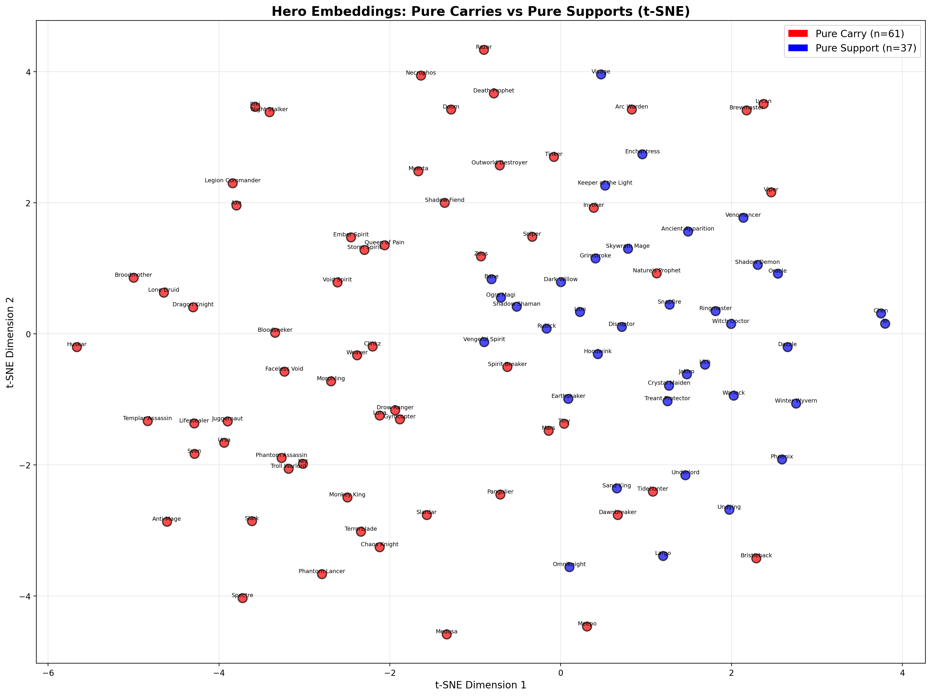
The first thing I noticed is that the carries and supports are cleanly separated. There is a region of the map where carries live and a region of the map where supports live. The model has independently learned that some heroes function as the late-game damage dealer and some heroes function as the early-game enabler, purely from how they pair with other heroes to win or lose games.
That alone would have been satisfying. But the second pass through the picture is when I genuinely sat back in my chair, because:
- Drow, Luna, and Gyrocopter form their own pocket. Classic ranged late-game agility carries.
- Terrorblade and Chaos Knight sit next to each other. The two iconic illusion carries.
- Juggernaut and Lifestealer cluster. Both have built-in spell immunity as part of their kit.
- Weaver and Clinkz are paired. Both invisible squishy carries with burst.
- Phantom Assassin, Kez, and Troll group up. Bursty melee carries.
- Riki and Night Stalker -- the gankers. Pickoff specialists.
- Ember Spirit, Storm Spirit, Void Spirit, and Queen of Pain form the bursty mids cluster.
- Shadow Demon and Oracle are essentially on top of each other -- the two iconic save supports.
- Necrophos, Doom, Death Prophet, and Razor cluster -- the "anti-carry" tanky midgame heroes that win the game by simply not dying while doing damage.
- Chen and Io sit off in their own corner together. Both are specialty supports almost nobody picks. They share a corner of embedding space because they share a corner of pick rate.
- Lion, Shadow Shaman, Rubick, Vengeful Spirit -- a chunk of supports each with a single-target stun or disable, all clustered in the middle.
None of those are labels I gave the model. The groupings are consistent with categories that Dota players use, arrived at by watching outcomes only.
I want to sit on this because it's easy to gloss over. The model's only signal is "this set of ten heroes won, that set of ten heroes lost." From that, with no help, it placed Weaver next to Clinkz, Drow next to Luna, and Chen next to Io. Those are relationships that take a Dota player years of pattern-matching to articulate, and the model arrived at them in 22 minutes of training without ever knowing the heroes had names.
Some of it I would not have predicted. The "anti-carry" grouping (Necrophos, Doom, Death Prophet, and Razor) matches a category real players use, but it isn't in any official tag -- it's a community thing.
The map isn't perfect. There are heroes I'd quibble with the placement of. But it looks coherent, and coherent is exactly what I should be suspicious of.
Making the Map Pay Rent
Here's the problem with everything I just wrote: t-SNE is extraordinarily easy to narrate.
It takes 128 dimensions and crushes them into two. That's lossy and non-linear, it has a perplexity knob that changes the picture, and it will produce some arrangement no matter what you feed it -- including noise. Meanwhile I've been playing this game for fifteen years and I know a hundred true things about every hero on that chart. Hand me any 2-D scatter of Dota heroes and I will find stories in it. That isn't a model discovering structure. That's me.
So before letting myself keep those paragraphs, I went and measured what I was actually claiming, in the 128-dimensional space the model really learned, with t-SNE nowhere in the room.
Do same-role heroes sit near each other? For each of the 98 unambiguous heroes, take its nearest neighbours by cosine distance and ask what fraction share its role. Then shuffle the role labels ten thousand times to see what that number looks like when there's nothing there.
| neighbours | same-role fraction | shuffled labels | z |
|---|---|---|---|
| 1 | 0.786 | 0.526 | +4.4 |
| 3 | 0.803 | 0.525 | +7.8 |
| 5 | 0.804 | 0.526 | +10.0 |
| 10 | 0.777 | 0.525 | +13.0 |
Can you read role straight off the vector? A logistic regression on the raw 128-d embeddings, stratified 5-fold, twenty repeats: 89.3% accuracy. Answering "carry" every time gets 62.2%, because there are more of them. The same probe on permuted labels gets 52.8%.
And the specific pairs I got excited about? This is the one I expected to lose. For every pair named in that bullet list, I asked where each hero sits in the other's full-space neighbour ranking, out of 126. Random pairing would put the median around 63.
The median is 2. Ninety-three percent of the pairs I named are inside each other's top ten neighbours. Juggernaut and Lifestealer are mutual nearest neighbours; so are Shadow Demon and Oracle; so are Chen and Io.
Two groups did worse, and both are informative. The bursty-mids cluster is solid for Ember, Storm and Queen of Pain, but Void Spirit's nearest neighbour is Puck -- which, if I'm honest, is a better answer than mine. And the "anti-carry" group is the loosest thing on the chart: median rank 4, with Necrophos's nearest neighbour being Leshrac and Doom's being Night Stalker. That's the cluster I was proudest of naming, and it's the one the numbers support least. Draw your own conclusions about my other names.
So the plot survives, with the emphasis moved. The role structure is real and it lives in the embedding, not in the projection. The projection is a way of looking at it.
Takeaway
The headline number from this whole exercise is 58.05%, but the headline number is not actually the headline. The headline is the map.
A model trained only to predict win probability, given only hero IDs and outcomes, learned a representation from which a hero's role is readable at 89% accuracy by a linear probe -- and in which the informal groupings players actually use, down to "illusion carries," turn out to be genuine neighbourhoods. Nobody put that there. It's what predicting the outcome required.
I want to be careful about the size of that claim, because the version I first wrote down was bigger. This is not evidence that the model understands Dota. It's evidence that the geometry it learned carries role information -- which is a real, measurable, checkable thing, and not the same as comprehension. The model still can't tell you what an ability does, and it has not yet been asked to do the one job I built it for.
So the earned version of the aphorism is narrower than the one I wanted: train a model to predict outcomes and you get, for free, a representation of whatever the outcomes depended on. That's not new -- it's the entire premise of representation learning. But there's a difference between knowing it as a textbook fact and watching it fall out of a 654k-match dataset of low-rank pub games, then going back and checking that it really did.
The model can tell a carry from a support. It has Juggernaut and Lifestealer as each other's closest relatives, and it thinks Chen and Io are the same kind of strange.
What the model does not yet know is whether any of this is going to help me win a game of Dota.
That's Part 5.